Data Model Building Practices for Business Intelligence
Having determined your data strategy (see Choosing a Data Strategy for Embedded Self-Service), you now need to set up your data model for self-service business intelligence (BI).
What is Self-Service BI?
Watch this video for an explanation of:
- The history of BI
- BI complexity
- Descriptive - what happened?
- Facts, anomalies, trends
- Diagnostic - why did it happen?
- Root causes, correlations, insights
- Predictive - what will happen next?
- What-if analysis, forecasting, optimization
- Prescriptive - what should be done next?
- Assisted Intelligence - automated processes for executing what should be done next
- Descriptive - what happened?
- BI life cycle
- Data producers
- Data pipeline
- Data consumers
- Dashboard life cycle
- Planning, execution, delivery
Data Modeling
When modeling data, BI recommends that you either use a flat or fact-dimension table schema:
- To implement a flat table schema, the user denormalizes all their data into a single table. Denormalizing data
requires extensive data duplication, and row duplication, resulting in an exponential growth of the database size.
Example:
Placing all product names in a sale transactions table will cause a duplication of strings in your data model.
- To implement a fact-dimension table schema, the user denormalizes some of their data and places it in a two-level
hierarchy model:
- The first level is the fact level (for measures). It is used to store transactional data that can be aggregated.
- The second level is the dimension level (for filters). It is used to store descriptive information about the transactions. This data is used for filtering or segmenting the data.
For an explanation of the data model types and how to create and manage them, see Introduction to Data Models.
Table Relationships
The logical connection between the tables is known as a table relationship. It is created by linking two related fields (keys), one from each table. When using multiple data tables in the model, a user must teach the system how to join them for handling cross-table queries.
Example:
If the fact table describes sale transactions and the dimension tables describes the products sold, the user may request the total sales of all red products.
A table relationship describes one of the following relations:
- A one-to-one relationship
- A one-to-many relationship
- A many-to-many relationship
Watch this video for a brief explanation of the three relations above:
Watch this video for a detailed explanation of data relationships:
One-to-One Relationships
The one-to-one relationship is a relationship where each value in the key column of table A exists either once or zero times in the key column of table B, and vice versa.
Example:
- A customer has a store membership; a store membership belongs to a single customer.
- A city is the capital of one country; a country may only have one capital.
- Each employee (identified by Employee ID) has one SSN; an SSN belongs to only one employee.
A one-to-one relationship is usually visualized as follows:

Each entry in table A appears only once in table B. Each entry in table B appears only once in table A.
One-to-Many Relationships
The one-to-many relationship is a relationship where each value in the key column of table A exists either once or zero times in the key column of table B, and each key column of table B may appear multiple times in the key column of table A.
Example:
- A person belongs to one family. However, the family includes multiple people.
- A car has one VIN; a VIN may only belong to one car.
- A person was born in a single hospital. However, many people were born in that hospital.
- An airplane is parked in a single airport. However, the airport accommodates multiple planes.
A one-to-many relationship is usually visualized as follows:

Many-to-Many Relationships
A many-to-many relationship is a relationship where each value in the key column of table A may appear multiple times in the key column of table B, and vice versa.
Example:
- A person belongs to multiple groups; a group contains multiple people.
- A product belongs to multiple categories; each category includes multiple products.
- A student participates in multiple classes; a class includes multiple students.
A many-to-many relationship is usually visualized as follows:

Many-to-Many Relationship Considerations
There are two types of many-to-many relationships:
- Expected many-to-many relationships
- Unexpected many-to-many relationships
The Expected Many-to-Many Relationship
In some cases, many-to-many relationships are expected and planned.
Example:
A company sets up fan groups and stores their data in the following user/group table schema:
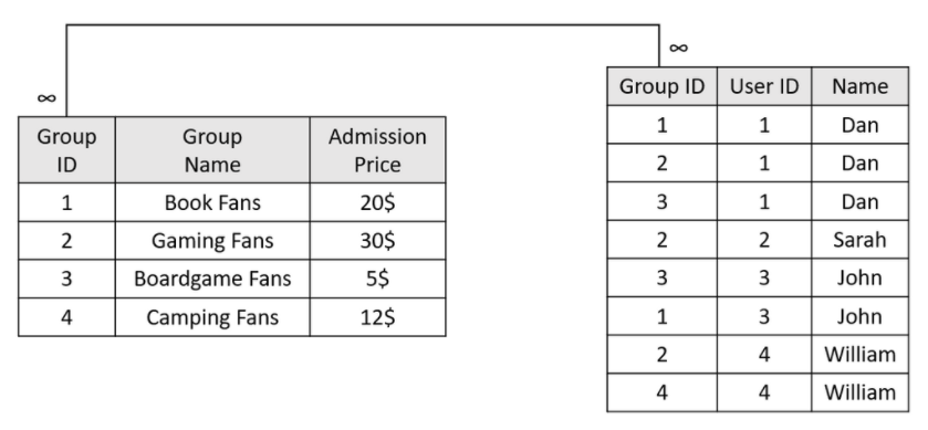
- To calculate Dan's monthly admission, both tables must be joined on the Group ID field, and filtered by Dan's name. The result is a sum aggregation of the Admission Price column, that is, $20 + $30 + $5 = $55.
- To calculate the number of people that participate in the Boardgame Fans group, both tables must be joined on the Group ID field, and filtered by the group's name. The result is a count aggregation of the User ID column, that is, 2 people.
- To calculate the total cash flow, the user table must be grouped by the Group ID, and the number of users per group must be counted. Then both tables must be joined on the Group ID field. The result is the sum of the user count x admission price, that is, $40 + $90 + $10 + $12 = $152.
The Unexpected Many-to-Many Relationship
In some cases, many-to-many relationships are created unexpectedly. This could happen due to an unexpected ("wrong") business question or inadequate data modeling.
Example:
Here is a retail use-case where a company stores purchases (from vendors) and sales (to customers):
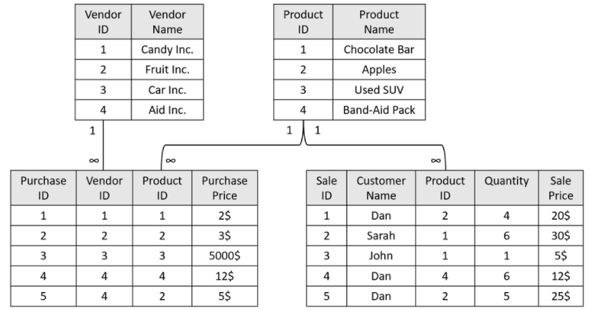
- To calculate the number of chocolate bars sold, the Purchases and Sales tables must be joined on the Product ID field, and filtered for chocolate bars. The result is a sum aggregation of the Quantity column, that is, 6 + 1 = 7.
- To calculate which customer spent the most, the Sales table must be grouped by customer name and a sum aggregation of the Sale Price must be calculated for each customer. The result is the maximal value, that is, Dan who spent $75.
- To calculate the number of sales made by Aid Inc. is probably an incorrect question as the company does not sell to vendors. Even so, given the question, Sisense will attempt to find a way to calculate this by joining the Vendors table with the Purchases table on Vendor ID and filtering by Aid Inc. It will then take the products found and join them against the Sales table. The result will be the sum of Sales Price, that is, $20 + $12 + $25 = $57, which is incorrect.
Thus, the risks of many-to-many mistakes may lead to:
- Displaying no data in your widget.
- Displaying incorrect data in your widget.
- Generating a huge JOIN operation, leading to excessive use of memory and/or computing power.
In severe cases, where data tables are huge, a many-to-many relationship may lead to an ElastiCube crash or a complete Sisense instance failure.
Dealing with Many-to-Many Relationships
There are two ways to deal with many-to-many relationships:
- Avoiding them
- Bullet-proofing your data model
Avoiding Many-to-Many Relationships
The easiest way to resolve many-to-many relationship-related issues is by avoiding them.
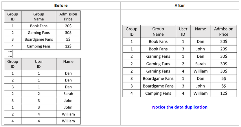
Avoiding these relationships is not necessarily easy. Doing so might be very expensive in terms of computing
resources (data transformation) and data storage (data duplication).
Example:
Bullet-Proofing Your Data Model
Another way to deal with many-to-many relationships and avoid their related risks is bullet-proofing the data model. There are a few simple practices you should follow to avoid errors originating from incorrect business questions (see Best Practices for Data Modeling),
Other Mitigation Steps
Expect the unexpected and plan ahead. Someone may unintentionally generate a many-to-many relationship and risk the Sisense instance stability. As a best practice, configure data groups. A data group configuration refers to the ability to pre-allocate resources towards an ElastiCube and/or limit the number of resources the ElastiCube can use.
Example:
You have 10 construction workers.
Scenario #1: You want to ensure that a single construction project does not use more than 5 workers.
Scenario #2: You want to ensure that an important construction project has 2 workers preallocated to it.
Scenario #3: You want to ensure that a single construction project has 2 workers preallocated, but does not use
more than 5 workers.
These settings allow prioritizing resources and ensuring that the right resources get the right QoS (Quality of
Service).
Best Practices for Data Modeling
In data modeling, a well-known issue to avoid is unexpected many-to-many relationships between tables in your data model. Where such many-to-many relationships exist, they can produce random or empty results, meaning that the end user may be making decisions based on potentially incorrect data. Hence, the need to avoid many-to-many relationships whenever possible. The following best practices help avoid these redundant relationships:
- Avoiding Random Paths & Cycles (see Avoid Dimension Table Cycles)
- Creating Optimal Table Relationships (see Table Relationships)
- Hiding & Dropping Columns (see Hide Irrelevant Columns)
- Correct Data Extraction (see Keep Data Extraction Costs in Mind)
- Fake and Surrogate Keys (see Link All Dimension Tables to All Fact Tables)
- Implementing data security as a dimension (see Data Access Security)
Watch this video about data modeling best practices:
Each best practice addresses a different data modeling mistake or potential "wrong" business question.
Use a Fact-Dimension Table Schema
BI best practices recommend using a two-level table hierarchy model, including:
- Facts (measures) - Containing data that is aggregated (e.g., a list of sale transactions).
- Dimensions (filters) - Describing the data inside the fact (e.g., a list of products and their characteristics).
Sisense recommends implementing the fact-dim schema structure because:
- A two-level table hierarchy model reduces the number of JOIN events during a query's execution. This results in a shorter query runtime, fewer computation operations, less memory consumption, and provides a better user experience.
- A two-level table hierarchy model simplifies the data model, making it easier to debug data inconsistencies and follow the query path.
- There is only one way to get from every fact to every dimension (and vice versa).
Data modeling is a task that requires much planning and may be very challenging. The rule of thumb when migrating your database structure into a fact-dim structure is to start by finding out what the business' questions are. Then, use the business questions to define which data is used for filtering and segmenting (dimensions) and which data is used for aggregations (facts). Modeling your data correctly is key to your dashboard's success (in terms of runtime performance and data accuracy).
Watch this video for an explanation about facts and dimensions:
Never Link a Fact Table to Another Fact Table
Two fact tables should never connect to each other. A fact table should only connect to dimension tables. Connecting two fact tables directly may lead to a JOIN between them, potentially causing a huge query to execute and crashing the ElastiCube.
Never Link a Dimension Table to Another Dimension Table
Two dimension tables should never connect to each other. A dimension table should only connect to fact tables. Dimension tables are used to describe the data in the fact table. Different dimension tables usually do not relate to each other and, if they do, linking them may lead to a table cycle (see Avoid Dimension Table Cycles).
Link All Dimension Tables to All Fact Tables
Every dimension table should be connected to all fact tables.
Every fact table should be connected to all dimension tables.
Every dimension field may be used for filtering and/or segmenting data. Every fact field may be used for aggregating data. Your user can choose to filter and aggregate any sets of fields, leading to a random path.
Some fact-dimension relationships are straightforward. Others are not.
Example:

Connecting the Product dimension to the fact tables is straightforward, as every sale and purchase event involves a
specific product. However, connecting the Vendor dimension table is not. A vendor does not participate in sale events.
To resolve this, create a fake key, allowing a relationship and ensuring that the tables either
always or never join.
Watch this video for an example of using fake keys:
For more information, see Fake Keys.
Consolidate One-to-One Dimension Tables
In some cases, you may have dimensions that connect on the same primary key. If two dimensions holding the same primary key have a one-to-one relationship, Sisense recommends consolidating them, to decrease the number of JOIN operations.
Example:
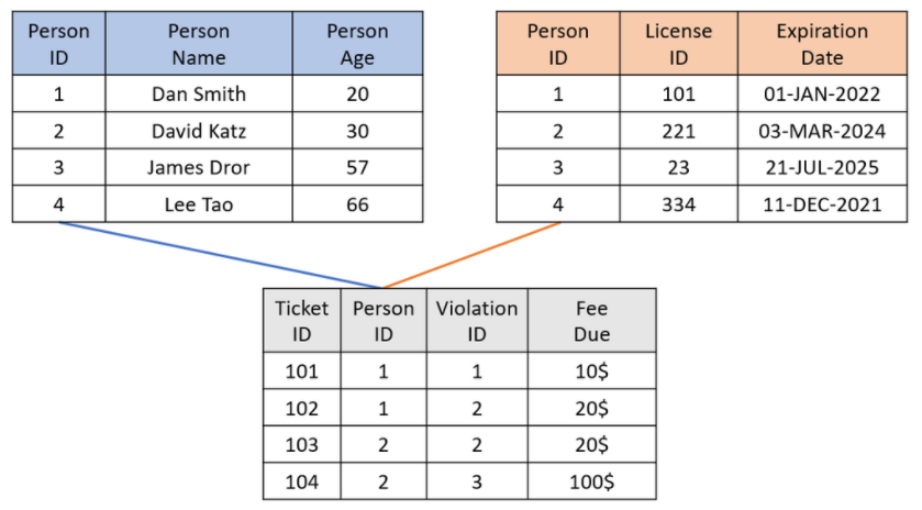
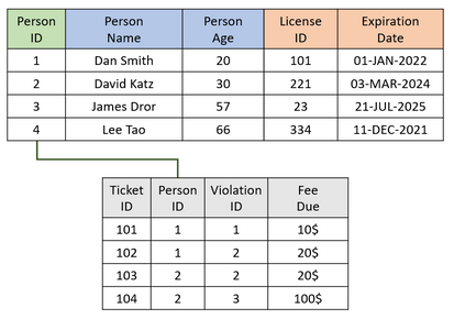
Assuming each person has one driver's license and each driver's license belongs to one person, the two dimensions
should be consolidated. By doing so, a dashboard attempting to filter tickets based on age range and license type
would require one less JOIN operation. This results in the following:
See Adding Custom Tables.
Hide Irrelevant Columns
In many cases, columns used for creating relationships (primary/foreign keys) are also public keys. But, if the end-user actually uses a User ID in his filtering, a dashboard designer may use the incorrect field name when creating a widget, leading to incorrect query results (many-to-many), and query failure in extreme cases.
Sisense recommends hiding key columns from the user whenever possible.
Example:
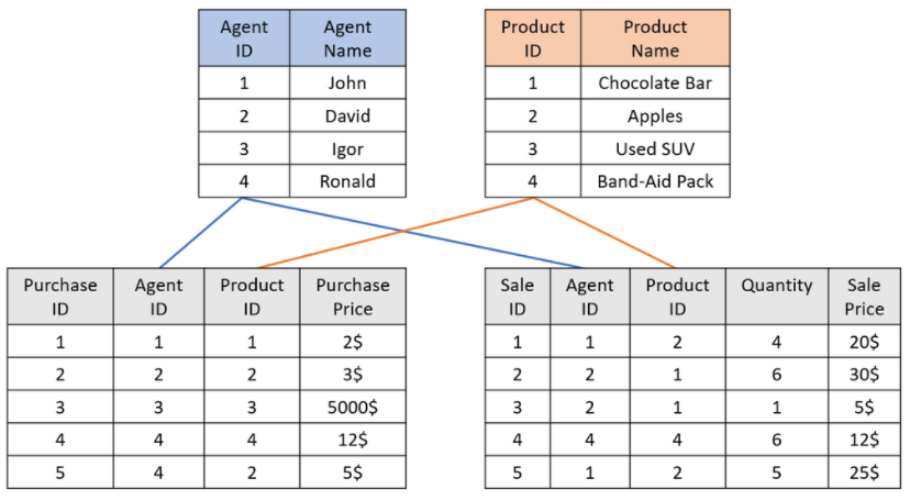
Scenario #1
The customer builds a widget to count the number of purchase transactions containing product #3:
- The aggregative field is Purchase ID (in the Fact_Purchases table).
- The filtering field is Product ID (mistakenly chosen from the Fact_Sales table).
- The result may be incorrect (e.g., if product #3 was never sold) and will require joining the two fact tables (a very expensive operation).
Scenario #2
The customer builds a widget to count the agents who sold apples:
- The filtering field is Product Name (in the Dim_Products table).
- The aggregation field is Agent ID (mistakenly chosen from the Dim_Agents table).
- The result will be unpredictable and most likely incorrect as there is no way to determine which fact table will be used for joining these two dimensions. This is known as a random path.
The solution for the example is as follows, where grayed-out fields are hiidden:
.png)
- In scenario #1, there is only one Product ID field.
- In scenario #2, there is only one Agent ID field.
Notice that the hidden fields align with the relevant business questions
See Managing Tables and Columns.
Avoid Dimension Table Cycles
The term Chaining Dimension Tables refers to a scenario where you connect a fact table to a dimension table, and then chain an additional dimension table to that table.
Sisense recommends avoiding table chaining whenever possible because this type of structure introduces unnecessary JOIN operations.
Example:
Try to count all red products sold.

Using this type of structure may also lead to cases where the data structure has a table cycle, leading to unexpected
query results - for example, trying to count all sales with a Red filter:
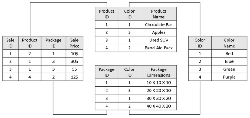
Table cycles can be resolved using various methods (depending on the business questions). Here are three possible solutions for this problem:
- Denormalize the Color Name and place it in both the Product and Package dimension tables. This will reduce one JOIN event per query and allow the user to choose between the two filters.
- Disconnect the color dimension from the packaging dimension. This is a valid solution if there are no business questions based on packaging color
- Duplicate the Color dimension, once for the product and once for packaging.
Validate Dimension Primary Keys
The primary keys of your dimension tables must be unique and not null. Making sure that the primary key is unique will guarantee a one-to-many relationship (rather than a many-to-many relationship).
Example:

Note the error in the Products dimension table - two items have the same Product ID. A simple query may result in a JOIN operation that requires twice the amount of work and, more importantly, gives an incorrect result.
To monitor your dimension tables, create a dup-check table that counts the following:
| Value | Definition | Expected Value |
|---|---|---|
| Key Count | The total number of keys |
|
| Unique Key Count | The number of unique keys | Should be equal to Key Count |
| Null Key Count | The number of NULL keys | Should be zero |
To create such a table, create a custom table with code similar to this:
   SELECT
      'Customers' AS Table_Name,
      COUNT(c.[CustomerID]) AS Key_Count,
      COUNT(DISTINCT(c.[CustomerID])) AS Distinct_Keys,
      SUM(CASE WHEN c.[CustomerID] IS NULL THEN 1 ELSE 0 END) AS Null_Keys
      FROM
      [dim_Customers] c

      UNION

      SELECT
      'Employees' AS Table_Name,
      COUNT(c.[EmployeeID]) AS Key_Count,
      COUNT(DISTINCT(c.[EmployeeID])) AS Distinct_Keys,
      SUM(CASE WHEN c.[EmployeeID] IS NULL THEN 1 ELSE 0 END) AS Null_Keys
      FROM
      [dim_Employees] e

      UNION

      ...
Naming Convention
BI best practices recommend naming the fact and dimension tables with a relevant prefix.
Example:
The Sale_Events table should be renamed to Fact_Sale_Events. The Employees table should be renamed to Dim_Emolyees.
This enables both the data modeler and dashboard designer to quickly identify the table type. By identifying the data correctly, you can avoid mistakes that would lead to incorrect data modeling.
To rename tables, see Managing Tables and Columns.
Create the Dup-Check and Dup-List Tables
BI best practices recommend verifying that the values in the dim_tables' keys are:
- Unique
- Not NULL
Two keys in a dimension table that hold the same value will result in incorrect widget results.
Example:
A product dimension table erroneously has the same product ID for two items, shirts and pants (both given the shirts
ID). You have a fact table that holds a list of sale events, each for a single product. The fact table includes a
dimension representing each product. Thus, sales for shirts and pants appear in the fact table as if they are sales of
shirts.
Counting the sales by product item will result in zero results (no pants were sold) or incorrect results (more
shirts were recorded as sold than were actually sold).
To verify dimension table key value uniqueness, add a custom Dup_Check table with the following SQL code:
      SELECT
      'Dim_Customers' AS Table_Name,
      COUNT(c.[CustomerID]) AS Key_Count,
      COUNT(DISTINCT(c.[CustomerID])) AS Distinct_Keys,
      SUM(CASE WHEN c.[CustomerID] IS NULL THEN 1 ELSE 0 END) AS Null_Keys
      FROM
      [dim_Customers] c
The Key_Count value should equal the Distinct_Keys value.
The Null_Keys value should be zero.
If a duplicate value was found, add an additional custom Dup_List table with the following SQL code:
      SELECT
      'Dim_Countries' AS Table_Name,
      c.[CountryID] AS KeyName,
      COUNT(c.[CountryID]) AS KeyCount
      FROM
      [dim_Countries] c
      GROUP BY
      c.[CountryID]
      HAVING
      COUNT(c.[CountryID]) > 1
The resulting list will contain the duplicate keys and the number of times they appear in the dimension table.
Avoid "SELECT *"
BI best practices recommend avoiding SELECT * statements when importing a table into Sisense.
Using the SELECT * statement is easy and straightforward. However, it has the following disadvantages:
- If a person adds a column to the source table, Sisense will not be aware of the change and will not import it. A manual Schema Refresh is required.
- If a person removes a column from the source table, Sisense will not be aware of the change and will still expect it during the build process. The build operation will fail and a manual Schema Refresh will be required.
To change the SQL query used to extract data, see Changing Connection Settings for Data Sources.
Keep Data Extraction Costs in Mind
BI best practices recommend avoiding data that you do not require from your databases. Three main reasons to only pull the data you need into your ElastiCube are:
- Cloud storage vendors' charging models may rely on either the amount of data queried and/or the computation power required to generate the data.
- Importing irrelevant data increases the overall size of the ElastiCube.
- Importing irrelevant data increases the build time.
To change the SQL query used to extract data, see Changing Connection Settings for Data Sources.
No More Than Five Lookup Columns per Table
BI best practices recommend enriching table data by using custom columns. If the data that must be enriched exists in other tables in the data model, it is recommended to use LOOKUP functions. When using multiple LOOKUP functions, consider generating a new custom table if more than five LOOKUP functions are needed.
LOOKUP functions are much more efficient at performing table scans than an SQL query. However, as custom columns are generated after the tables are created, having multiple LOOKUP functions may lead to a long build time. In this case, it might be more efficient to create a custom table with the right query rather than performing multiple scans. See Adding Custom Tables.