Enhancing Data
Last updated: June 11, 2026
| Tier | Deployment |
|
|
|
Note:
The images on this page were taken in the desktop version of Sisense, however, the same principles described on this page also apply to the online version of Sisense.
The following examples explain how to add attributes and / or records that did not exist in the data source.
Calculating Derived Facts
Business Case
Derived Facts are additional facts that we calculate while importing or delivering the data. For example:
Modeling Challenge
You must decide whether to calculate the derived facts on demand, meaning in the web application, or in advance in the ElastiCube. Take into consideration that calculating "On Demand" Derived Facts in the web application can enable more dynamic filtering, while calculating them in the ElastiCube stage will save query time when retrieving the data, and enforce calculation consistency, especially with non-trivial facts. This is due to the fact that the dashboard designer / end users will receive consistent results for measures, instead of having to create the complex measures individually, by their own understanding.
Solution
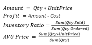
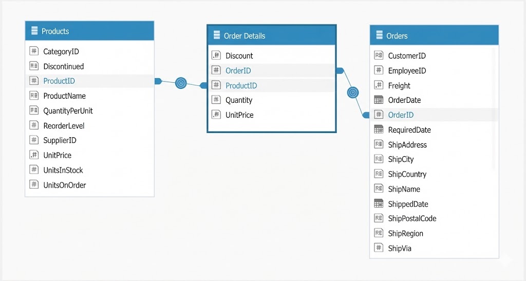
In the following schema you can create a derived fact to calculate the inventory ratio per product.
Create a Adding Custom Tables using an SQL Expression that joins the Order Details table with the Products table and returns the division result of Quantity and UnitOnOrder, with the following Syntax:
SELECT
[Products].ProductID,
tofloat(sum(UnitsOnOrder))/tofloat(sum(Quantity)) AS InventoryRatio
FROM [Products] JOIN [Order Details]
ON [Products].ProductID=[Order Details].ProductID
GROUP BY [Products].ProductID
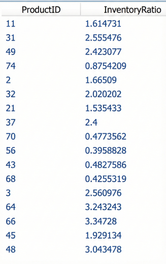
HAVING tofloat(sum(UnitsOnOrder))/tofloat(sum(Quantity))>0The result table will give the desired results:
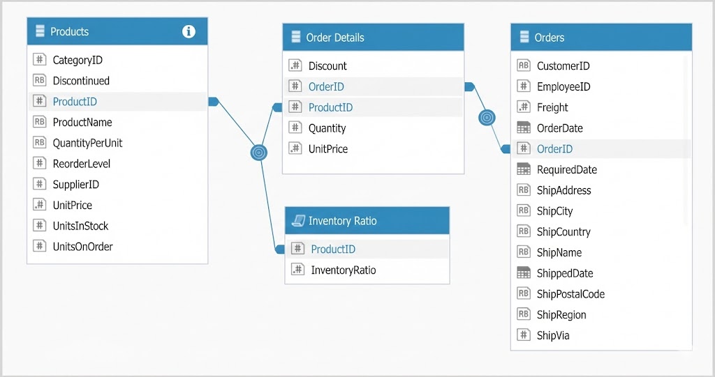
Connect the custom table to the rest of the tables:
Note:
You can also add the InventoryRatio measure to the Products table using the Lookup() function by ProductID.
Calendar vs. Fiscal Year
Business Case
A large number of companies use a fiscal calendar that does not comply with the Gregorian 12-month calendar.
Modeling Challenge
This requires modeling the data properly so that the data can be reported or analyzed via the normal calendar or via the revised fiscal calendar.
Solution
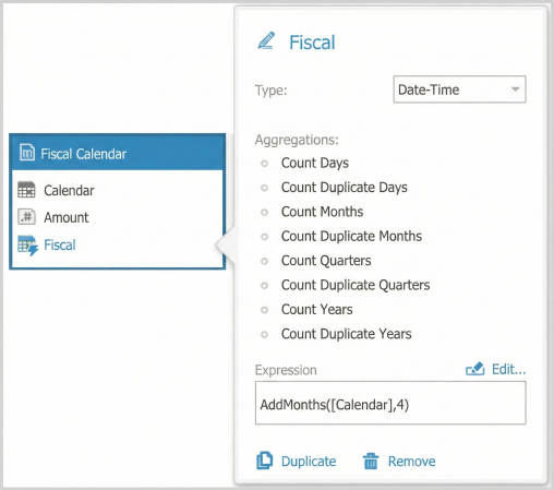
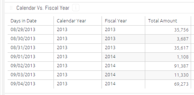
In this example, assume that the Fiscal Calendar starts on September 1st. So if we are in the calendar year of 2013, then the fiscal year of 2014 starts September 1st. To accomplish this, we create a custom field that takes the date field and adds four months to it.
When you create a pivot table in the web application, you will see that the new year (2014) starts in September using the Fiscal Year field.
Time Zone Conversion
Business Case
In many cases, we need to generate reports based on data from different time zones.
Modeling Challenge
When working with different time zones, the challenge is to store all of the business transactions in an absolute time reference that does not change with the seasons, locations (for instance - GMT), or daylight saving. Therefore, the absolute transition time is a combination of location and date.
Solution
The aim is to add an Absolute Time field to every business transaction, based on its location and time.
Step 1 - Create a Reference Source Table
Create a source table (database table / Excel / CSV) that contains the countries and cities that exist in the database, a numeric representation of timestamp range to determine if the transaction belongs to daylight savings time or not, and the UTC to allow the conversion to GMT.
For example:
| Country | City | DST_From | DST_To | UTC |
| USA | Seattle | 20120311.2 | 20121103.1 | -7 |
| USA | Seattle | 20121103.1 | 20130310.2 | -8 |
| USA | Seattle | 20130310.2 | 20131027.1 | -7 |
| USA | Seattle | 20131027.1 | 20140309.2 | -8 |
| UK | London | 20120325.1 | 20121028.2 | 0 |
| UK | London | 20121028.2 | 20130330.1 | 1 |
| UK | London | 20130330.1 | 20131027.2 | 0 |
| UK | London | 20131027.2 | 20140330.1 | 1 |
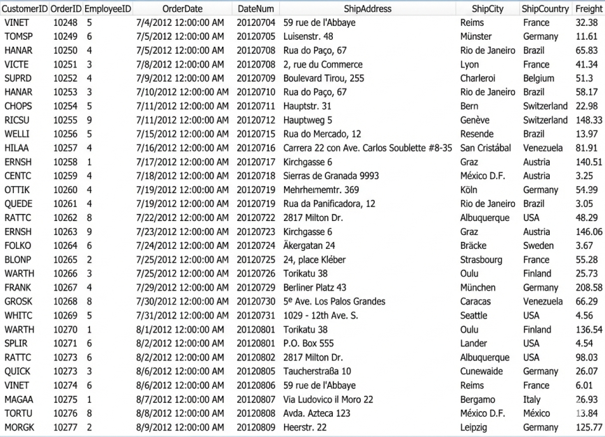
Step 2 - Add a Numeric Representation of the OrderDate
To associate the Order Date with its UTC, create a custom field of type Decimal with a numeric representation of the Date timestamp, using this SQL statement:
getyear(OrderDate)*10000+getmonth(OrderDate)*100+getday(OrderDate)+ToDouble(gethour(OrderDate))/100 The result table should look like this:
Step 3 - Join between the Two Tables
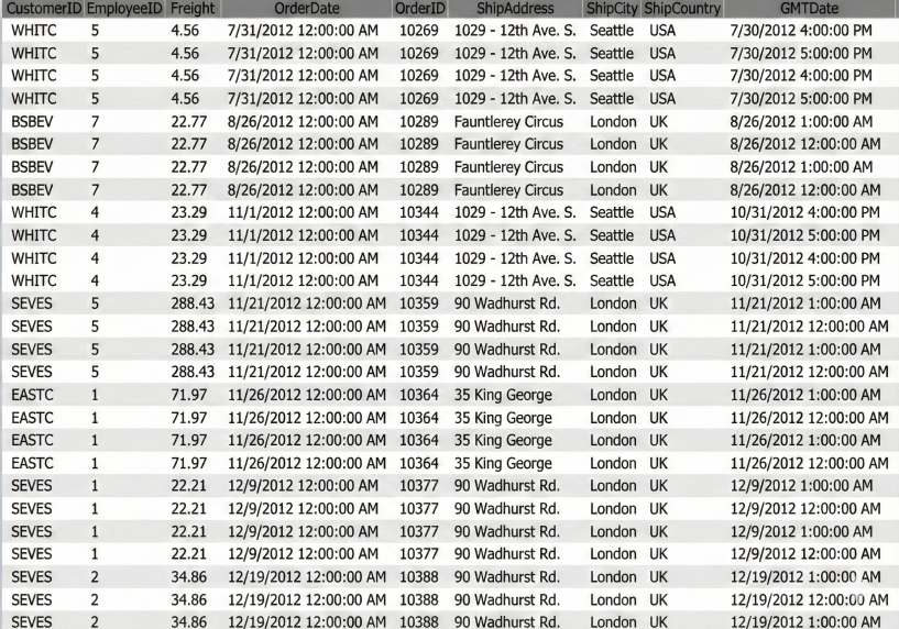
The third step includes creating a custom SQL expression that joins between the two tables and creating the Absolute Time custom field within it (GMTDate). This is to create a synchronization between all the transactions.
The custom field will be created using the add hours function with the matching UTC value. See the following script:
         SELECT
         [Orders].CustomerID,
         [Orders].EmployeeID,
         [Orders].Freight,
         [Orders].OrderDate,
         [Orders].OrderID,
         [Orders].ShipAddress,
         [Orders].ShipCity,
         [Orders].ShipCountry,
         AddHours(([Orders].OrderDate),[GMT Conversion.csv].UTC) AS GMTDate
         FROM [Orders]
         JOIN
         [GMT Conversion.csv]
         ON
         [Orders].ShipCity=[GMT Conversion.csv].City AND
         [Orders].ShipCountry=[GMT Conversion.csv].Country AND
         [Orders].DateNum>=[GMT Conversion.csv].DST_From AND
         [Orders].DateNum<[GMT Conversion.csv].DST_To
The result table will look like this:
Step 4 - Make Schema Adjustments
For the next step, do the following:
- Replace the current Orders table with the new one,
- Refer to the new Absolute Time custom field (GMTDate) as the leading date field
- Make the reference tables (Orders and GMT Conversion.csv) invisible.
Currency Conversion
Business Case
Most data for entities is recorded in their local reporting currency (i.e. $ for United States, £ for UK). Here we want to convert all the amounts to USD.
Modeling Challenge
This requires determining the Currency Rate of the region and then multiplying the value in local currency by the associated Exchange Rate by Month.
Solution
Create two custom fields in the GL Entries. The first will look up the Currency code of the region. This field will be used along with a month field to link to the Exchange Rates table.
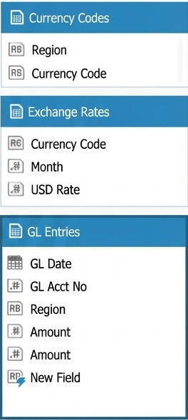
The first field in the GL Entries is created using the LOOKUP function to retrieve values from the Currency Codes table.
Lookup([Currency Codes],[Currency Code],Region,Region) Then create a second Custom Field for the Month of the GL Date.
GetMonth([GL Date]) Next, link the fields together (note that both Month fields were set to Integer and the Currency Codes table to Invisible).
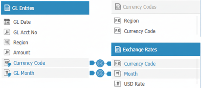
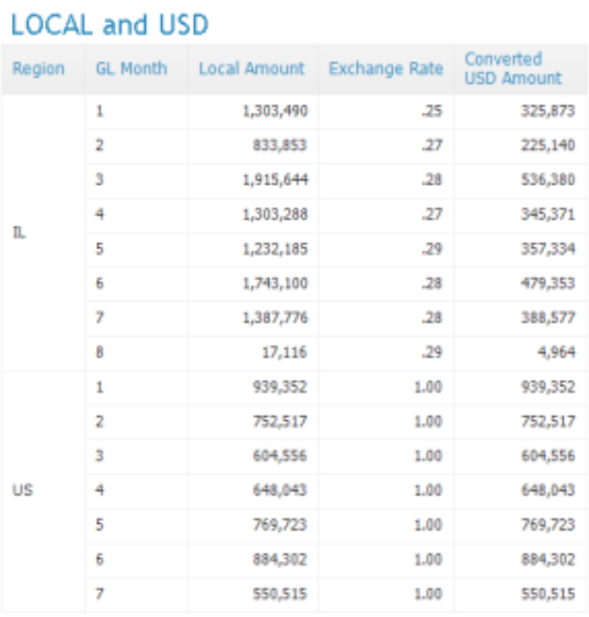
The Local Amount multiplied by the Exchange Rate gives the Converted USD Amount.
Current vs. Previous Period for Specific Date Range
Business Case
In many cases you might want to compare your business' performance last week, to the week before, or maybe see a percentage of sales growth for the current month/quarter compared to the previous month/quarter.
Modeling Challenge
Since we want the compared time range to be as flexible as possible, the solution has to include both layers - ElastiCube and web application.
Solution
Create a custom table in the ElastiCube to summarize the totals / counts per day for the source table:
             SELECT
             a.Date,
             sum(a.Revenue)AS value
             FROM [Accord 2011 Client List] AS a GROUP BY a.Date
Create a custom table in the ElastiCube with current vs. previous values, by adjusting the script below:
             SELECT
             curr.Date AS date,
             curr.value AS current,
             prev.value AS prev
             FROM [sum] curr
             LEFT JOIN [sum] AS prev
             ON curr.Date = addyears(prev.Date,1)
             UNION
             SELECT
             addyears(prev.Date,1) AS date,
             curr.value,
             prev.value
             FROM [sum] prev
             LEFT JOIN [sum] AS curr
             ON prev.Date= addyears(curr.Date,-1)
In the web application, add a date range picker using the days from the custom table. Then add two new numeric indicators. In the first numeric picker, add the "sum of the current value", in the second numeric picker, add the "sum of the previous value".
In the date range picker, select the days of interest and you will see the current and previous values.
Calculating the Number of Open Orders per Day
Business Case
An open sales order is where the order has been placed but has not yet been delivered. If for example there is an order for 100 items and against this order only 50 items have been delivered (it is partially delivered). A high level of open orders per day may indicate that something is wrong with orders handling.
Modeling Challenge
We cannot just count the number of orders per day because it will exclude orders that were open on a certain day and are already closed. Therefore, we will need to create a snapshot of the number of open orders per day.
Solution
-
Import an Excel file with all dates listed in the Orders table into the ElastiCube.
-
To improve query performance, convert all the date fields into numeric representations (for more information, see Numeric Representation of Date Fields).
-
Create the following custom table:
SELECT
s.Dates,
tm.Created_At,
tm.Closed_At,
tm.TicketId
FROM [All Dates] s LEFT JOIN [Orders] tm
ON s.DateInt >= tm.CreatedAtInt
AND (tm.SolvedAt IS NULL OR s.DateInt <= tm.SolvedAtInt)
Slowly Changing Dimensions
Business Case
Transactional data typically does not change, however the data that describes the associated dimensions may change. This example demonstrates how to manage dimensions that may be updated with new values within the data warehouse at different points in time.
For example, a customer that was living in NYC and moved to LA earlier this year.
DateCustomerCity
1/1/2011John SmithNYC
1/1/2013John SmithLA
Modeling Challenge
Following the example above, when the transactions were made last year, the customer was living in NYC. Later this year, the customer moved to LA.
If you decide to refer only to the last city and summarize revenue by city, the NYC transaction will be credited to LA only because the customer currently lives there.
If you connect the Customer field within the above table to the Customer field in the fact table, you will create a many-to-many relationship because Customer is not a unique identifier of this table.
Solution
The solution is to change the level of granularity of the Customer_City table and add the Date field to the key -
- Concatenation of the Slowly Changing Dimension table's unique identifier (for example - Customer_ID + Date)
- Creation of the same concatenated field in the transactions table.
- Merge between the 2 keys.
- This way, you can associate the [Customer_ID + Date] key of every transaction with the relevant customer city.